S3 API cost estimation in multi-tenant AWS S3 buckets

 SaaS providers with multi-tenant setups use cloud services to easily scale their workloads as more customers join. As they grow, it's crucial to keep an eye on each customer's API usage to allocate resources properly. By tracking API usage per customer, a company can tweak its pricing model or plan its budget more effectively. Sometimes, customers might be charged differently based on how many requests they make.

Many organizations using multi-tenant architectures turn to AWS for help with tracking and assigning costs to individual customers. SaaS providers often store customer data in unique sections within the same Amazon S3 bucket, which makes scaling easier and allows them to use various AWS services for data processing without needing a separate bucket for each customer.

In this guide, we'll show you how to estimate customer usage of Amazon S3 API calls in a multi-tenant environment using bucket prefixes. We'll use Amazon S3 Inventory to collect object metadata, AWS Lambda and Amazon EventBridge to schedule daily data aggregation, and Amazon Athena to query the data. This setup will give you insight into your customers' cloud API usage, helping you adjust your business model, improve forecasting, and charge customers more accurately.

AWS offers plenty of tools to help you understand and analyze service costs. For instance, Amazon S3 has cost allocation tags that you can attach to buckets. These tags help organize your resources in cost reports, allowing you to assign costs to different departments or teams. However, while you can tag the bucket prefix, these tags can't be used for cost allocation.

To accurately track and allocate API call costs in a multi-tenant bucket, follow these steps:

1. Use the Amazon S3 Inventory report to gather bucket metadata.
2. Set up an Amazon Athena S3 output folder and prepare database objects for tenant data.
3. Store and analyze Amazon S3 server access logs.
4. Create an AWS Lambda function to run daily after the S3 inventory report is generated, and schedule it with Amazon EventBridge to ensure it runs every day.
5. Create a ready-to-use view in Athena for easy access.

To show how this works, we set up a sample environment. In this example bucket, each prefix stands for a different customer. As you can see in Figure 1, each prefix contains a different number of objects, and each object has its own size.

Figure 1: Single bucket with multiple tenants (prefixes)

In Figure 2, you can see some of the contents of one of the prefixes in the aforementioned bucket.

Figure 2: Content of the prefix “customer_id=1/”

Our first task is to list all the objects in the bucket. While we could use the ListObjects S3 API, Amazon S3 Inventory is a more efficient way to do this. This feature creates a list of all the objects and their metadata in an S3 bucket. You can set Amazon S3 Inventory reports to run daily or weekly. To enable it, go to your S3 bucket, select Management, and then click on Create Inventory Configuration under Inventory Configuration. Choose the Daily frequency option.

Figure 3: Amazon S3 Inventory configuration

Important: To keep inventory data costs down and ensure fast queries, store the inventory report in Apache Parquet format.

To accurately track costs, we need to query our inventory report daily to spot any changes in the storage of our prefixes, which contain our customer data. We use the Amazon S3 Inventory report to pull the necessary information and store it in an external table for querying.

Remember, Amazon S3 Inventory reports capture a snapshot of the objects in a bucket at the time the report is created. This means some objects might be added or deleted between report generations.

To work with Athena tables, we need to set up an Athena database, which organizes tables logically. You can find more details on creating the database in the documentation.

CREATE DATABASE S3_pricing


CREATE EXTERNAL TABLE s3_inventory_report(
         bucket string,
         key string,
         version_id string,
         is_latest boolean,
         is_delete_marker boolean,
         size bigint,
         last_modified_date timestamp,
         e_tag string,
         storage_class string,
         is_multipart_uploaded boolean,
         replication_status string,
         encryption_status string,
         object_lock_retain_until_date bigint,
         object_lock_mode string,
         object_lock_legal_hold_status string,
         intelligent_tiering_access_tier string,
         bucket_key_status string,
         checksum_algorithm string,
         object_access_control_list string,
         object_owner string
) PARTITIONED BY (
        dt string
)
ROW FORMAT SERDE 'org.apache.hadoop.hive.ql.io.parquet.serde.ParquetHiveSerDe'
  STORED AS INPUTFORMAT 'org.apache.hadoop.hive.ql.io.SymlinkTextInputFormat'
  OUTPUTFORMAT 'org.apache.hadoop.hive.ql.io.IgnoreKeyTextOutputFormat'
  LOCATION 's3://INVENTORY_BUCKET/hive/'
  TBLPROPERTIES (
    "projection.enabled" = "true",
    "projection.dt.type" = "date",
    "projection.dt.format" = "yyyy-MM-dd-HH-mm",
    "projection.dt.range" = "2023-10-10-00-00,NOW",
    "projection.dt.interval" = "1",
    "projection.dt.interval.unit" = "DAYS"
  );

Note!!! Replace the 2022-01-01-00-00 date under projection.dt.range with the first day of the time range within which you partition the data in Athena. Replace s3://INVENTORY_BUCKET/ with the correct inventory location. After creating the table, run “MSCK Repair table” command. Otherwise you get an empty result set for the query. Read about this command in this documentation.

We turn on S3 server access logs to get detailed records of all the API requests made to our S3 bucket. You enable this feature at the bucket level, and the logs are delivered for free on a best-effort basis. These logs help you keep track of the requests made to your bucket. This free feature gives you enough accuracy to estimate the costs for your customers in a shared bucket.

Figure 4: S3 server access logs are delivered on a best effort basis

Whenever a user does something like GET, PUT, or LIST, it costs money based on the S3 pricing guide. We can use these logs to figure out the request costs for each prefix and customer. To follow along, you’ll need to enable S3 server access logs. Just open the bucket you want, go to the "Properties" tab, and switch "Server access logging" to "Enable."

Figure 5: Enable S3 server access logging

When you enable S3 server access logs, you need to specify a different S3 bucket for storing the logs. Don’t use the same bucket you’re monitoring, or you’ll create an infinite loop of log entries. Instead, create a new bucket to store the access log objects.

To manage storage costs in your new log bucket, we suggest setting up an S3 Lifecycle rule to automatically delete old logs.

Server access logs are similar to traditional web server access logs, so we’ll use Amazon Athena to analyze them. Follow the same process outlined here to format the data correctly. Start by creating a table to hold the initial log data, with each log entry in a separate column.

CREATE EXTERNAL TABLE s3_raw_logs (
`bucketowner` STRING,
`bucket_name` STRING,
`requestdatetime` STRING,
`remoteip` STRING,
`requester` STRING,
`requestid` STRING,
`operation` STRING,
`key` STRING,
`request_uri` STRING,
`httpstatus` STRING,
`errorcode` STRING,
`bytessent` BIGINT,
`objectsize` BIGINT,
`totaltime` STRING,
`turnaroundtime` STRING,
`referrer` STRING,
`useragent` STRING,
`versionid` STRING,
`hostid` STRING,
`sigv` STRING,
`ciphersuite` STRING,
`authtype` STRING,
`endpoint` STRING,
`tlsversion` STRING,
`accesspointarn` STRING,
`aclrequired` STRING)
ROW FORMAT SERDE
'org.apache.hadoop.hive.serde2.RegexSerDe'
WITH SERDEPROPERTIES (
'input.regex'='([^ ]*) ([^ ]*) \\[(.*?)\\] ([^ ]*) ([^ ]*)
([^ ]*) ([^ ]*) ([^ ]*) (\"[^\"]*\"|-) (-|[0-9]*) ([^ ]*)
([^ ]*) ([^ ]*) ([^ ]*) ([^ ]*) ([^ ]*) (\"[^\"]*\"|-)
([^ ]*)(?: ([^ ]*) ([^ ]*) ([^ ]*) ([^ ]*) ([^ ]*) ([^ ]*)
([^ ]*) ([^ ]*))?.*$')
STORED AS INPUTFORMAT
'org.apache.hadoop.mapred.TextInputFormat'
OUTPUTFORMAT
'org.apache.hadoop.hive.ql.io.HiveIgnoreKeyTextOutputFormat'
LOCATION
's3://ACCESS-LOG-LOCATION/'

Note: You will need to replace “s3://ACCESS-LOG-LOCATION/“ by the real S3 location that you used when you enabled S3 Server Access Logging.

Once we whip up this table and run a query on s3_raw_logs, we’re hit with loads of data. But hey, not all of it fits our cost allocation project's vibe, so we're ditching those extra columns. Gonna tweak the data a bit to make it more palatable. Also, that datetime field? It’s hanging out as a string right now. We’ll need to flip it to a datetime type if we want to group the data by date.

Figure 6: Query S3 access log results

We create a new table, to separate all of our manipulation from the row data table. For this, we create a new table:

CREATE EXTERNAL TABLE s3_access_cost_per_tenant
(
bucket_name string,
requestdatetime timestamp,
remoteip string,
requester string,
operation string,
customer_id string,
object_name string,
request_uri string,
isaccelerated int
)
PARTITIONED BY (access_log_date date)
STORED AS PARQUET
LOCATION 's3://S3-PROCESSED-S3_ACCESS-DATA/';

You should replace 's3://S3-PROCESSED-S3_ACCESS-DATA/' with the correct location for your environment. After inserting into the table, run MSCK Repair table s3_accesss_cost_per_tenant. Otherwise, you get an empty result set for the query. 

We now insert modified data into this table

insert into s3_access_cost_per_tenant
select bucket_name,
CAST(parse_datetime(requestdatetime,'dd/MMM/yyyy:HH:mm:ss Z') as timestamp) requestdatetime,
remoteip,
requester,
operation,
substr(url_decode(url_decode(key)),1,strpos(url_decode(url_decode(key)),'/')) customer_id,
substr(url_decode(url_decode(key)),strpos(url_decode(url_decode(key)),'/')+1) object_name,
url_decode(request_uri) request_uri,
case when endpoint like '%s3-accelerate%' then 1 else 0
end isaccelerated,
cast(date_trunc('day',date_parse(requestdatetime,'%d/%b/%Y:%H:%i:%S +0000')) as date) as access_log_date
from s3_raw_logs

Figure 7: Cost per tenant results after we cleaned the data.

Alright, things are looking clearer now. We ditched the irrelevant fields in this blog’s context and changed up some columns to make our future number crunching easier. Here's the plan: let’s hook up Amazon EventBridge to kick off AWS Lambda every day. Lambda can then update our aggregation table with the latest data from the previous day. Right now, Lambda's runtime is set at three seconds, but we're thinking of bumping that up to 30 seconds

Figure 8: Lambda Timeout settings

You can find a basic example of invoking an Amazon Athena query from Python, including the AWS Identity and Access Management (IAM) permissions needed, on AWS re:Post.

Here is the AWS Lambda function to update the aggregation table with last-day data:

from datetime import datetime
import time

import boto3

ATHENA_CLIENT = boto3.client("athena")


def create_queries():
    insert_query = (
        "insert into s3_access_cost_per_tenant "
        "select bucket_name,"
        "CAST(parse_datetime(requestdatetime,'dd/MMM/yyyy:HH:mm:ss Z') as timestamp)  requestdatetime, "
        "remoteip, "
        "requester, "
        "operation,"
        "substr(url_decode(url_decode(key)),1,strpos(url_decode(url_decode(key)),'/')) customer_id, "
        "substr(url_decode(url_decode(key)),strpos(url_decode(url_decode(key)),'/')+1) object_name, "
        "url_decode(request_uri) request_uri, "
        "case when endpoint like '%s3-accelerate%' then 1 else 0 "
        "end isaccelerated, "
        "cast(date_trunc('day',date_parse(requestdatetime,'%d/%b/%Y:%H:%i:%S +0000')) as date) as access_log_date "
        "from s3_raw_logs "
        f"where cast(date_trunc('day',date_parse(requestdatetime,'%d/%b/%Y:%H:%i:%S +0000')) as date) = cast(date_trunc('day',date_parse('{datetime.now().strftime('%Y-%m-%d 01-00')}','%Y-%m-%d %H-%i')) as date) "
        
    )
    return [
        "MSCK REPAIR TABLE s3_raw_logs",
        insert_query,
    ]


def execute_query(query):
    print(query)
    response = ATHENA_CLIENT.start_query_execution(
        QueryString=query,
        QueryExecutionContext={"Database": "s3_pricing"},
        ResultConfiguration={"OutputLocation": "s3://s3-blog-athena-result/"},
    )
    return response["QueryExecutionId"]


def wait_for_query_to_complete(query_execution_id):
    while True:
        response_query_execution = ATHENA_CLIENT.get_query_execution(
            QueryExecutionId=query_execution_id
        )
        state = response_query_execution["QueryExecution"]["Status"]["State"]

        if state in ("FAILED", "CANCELLED"):
            print(response_query_execution)
            raise Exception(f"Query did not succeed; state = {state}")
        elif state == "SUCCEEDED":
            print("Query succeeded")
            return

        time.sleep(1)


def lambda_handler(event, context):
    for query in create_queries():
        query_execution_id = execute_query(query)
        wait_for_query_to_complete(query_execution_id)

We'll mainly look at the "operation" part. It shows the API calls made on our stuff and helps us figure out the costs based on what operation was done and the storage type of the stuff involved. Check out the "Requests & data retrievals" section on the S3 pricing page for specifics on charges for different types of API calls depending on the storage type.

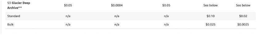
Figure 9: Amazon S3 pricing page for Requests and Data Retrievals in us-east-1

In our sample project, we observed the following API calls under the “operation” column:

REST.GET.ENCRYPTION

REST.GET.POLICY_STATUS

REST.GET.LOCATION

REST.GET.LOGGING_STATUS

REST.GET.VERSIONING

REST.GET.TAGGING

REST.GET.REPLICATION

REST.GET.OBJECT_LOCK_CONFIGURATION

REST.GET.BUCKETPOLICY

REST.GET.BUCKET

REST.GET.BUCKETVERSIONS

REST.GET.LIFECYCLE

REST.GET.WEBSITE

REST.GET.PUBLIC_ACCESS_BLOCK

REST.GET.ACLREST.GET.OWNERSHIP_CONTROLS

REST.GET.ANALYTICS

REST.GET.POLICY_STATUS

REST.GET.OBJECT

REST.GET.CORS

REST.GET.OBJECT_TAGGING

REST.GET.NOTIFICATION

REST.GET.ACCELERATE

REST.GET.INVENTORY

REST.GET.INTELLIGENT_TIERING

REST.GET.WEBSITE

REST.HEAD.BUCKET

REST.GET.REQUEST_PAYMENT

BATCH.DELETE.OBJECT

REST.OPTIONS.PREFLIGHT

REST.COPY.OBJECT

REST.COPY.PART_GET

REST.COPY.OBJECT_GET

REST.POST.MULTI_OBJECT_DELETE

REST.POST.UPLOADS

REST.POST.RESTORE

REST.PUT.ACCELERATE

REST.PUT.INVENTORY

REST.PUT.PART

REST.PUT.LIFECYCLE

REST.PUT.LOGGING_STATUS

REST.POST.MULTI_OBJECT_DELETE

REST.PUT.OBJECT

REST.PUT.BUCKETPOLICY

REST.PUT.VERSIONING

S3.CREATE.DELETEMARKER

S3.TRANSITION_SIA.OBJECT

S3.TRANSITION_ZIA.OBJECT

S3.TRANSITION_INT.OBJECT

S3.TRANSITION_GIR.OBJECT

S3.TRANSITION.OBJECT

S3.TRANSITION_GDA.OBJECT

S3.DELETE.UPLOAD

S3.RESTORE.OBJECT

S3.EXPIRE.OBJECT

Note: This is only partial list of operations available in Amazon S3

The requests that start with “S3.” are S3 Lifecycle transition operations and are priced according to the third column of the table in Figure 7.

Let’s explore the data by running the following Athena query:

select *
from s3_access_cost_per_tenant

Figure 10: Sample query results against s3_access_cost_per-tenant table

Once we run this query, you'll notice that the "customer_id" and "object_size" columns are blank. Checking the "requester" field reveals that these actions were carried out by AWS services such as Amazon Config or Amazon Macie. If your S3 bucket interacts with many other AWS services, expect to see numerous requests from them too. Internal S3 operations often lack specific object details.

Although these operations count as API requests, we're focusing on understanding the cost per prefix for now, so we'll set them aside. We'll discuss how to handle these special requests later.

Now, we've got all the data we need for our Athena queries to divvy up the request costs per customer. Looking at the pricing table, requests are billed per 1000 requests. So, our first step is to figure out how many requests we have for each tier. While the access log doesn't have storage info, the inventory data does. Thus, we need to merge the two tables to get our result.

Additionally, it’s very important that we need to consider the following storage tiers:

GLACIER

DEEP_ARCHIVE

STANDARD

INTELLIGENT_TIERING

STANDARD_IA

GLACIER_IR

ONEZONE_IA

Note!!! All the prices are taken from the official AWS Price List in the Northern Virginia region and are correct as of the date of this blog.

We will refer to the GET, SELECT and all other requests as category1 (cat1), PUT, COPY, POST, LIST as category2 (cat2), and S3 lifecycle as category3 (cat3). It is referenced in the column names of the following SQL statement.

select sa.customer_id,
sum (case
when sa.operation in ('REST.GET.OBJECT',
                      'REST.GET.BUCKET') and
                  sc.storage_class ='STANDARD' then 1
      else 0
end )/1000*0.0055 as standard_req_num_cat1,
sum (case
when sa.operation in ('REST.GET.OBJECT',
                      'REST.GET.BUCKET') and
                  sc.storage_class ='INTELLIGENT_TIERING' then 1
else 0
end )/1000*0.0055 as intel_req_num_cat1,
sum (case
when sa.operation in ('REST.COPY.OBJECT',
                      'REST.POST.UPLOADS') and
                  sc.storage_class ='STANDARD_IA' then 1
else 0
end )/1000*0.001 as standard_ia_req_num_cat2,
sum (case
when sa.operation in ('REST.COPY.OBJECT',
                      'REST.POST.UPLOADS') and
                   sc.storage_class ='GLACIER_IR' then 1
else 0
end )/1000*0.01 as glacier_ir_req_num_cat2,
sum (case
when sa.operation in ('S3.TRANSITION.OBJECT',
                      'S3.TRANSITION_INT.OBJECT') and 
                  sc.storage_class ='INTELLIGENT_TIERING' then 1
else 0
end ) as intel_req_num_cat3,
sum (case
when sa.operation in ('S3.TRANSITION_GDA.OBJECT',
                      'S3.TRANSITION.OBJECT') and
                  sc.storage_class ='DEEP_ARCHIVE' then 1
else 0
end ) as glacier_deep_arc_req_num_cat3
from s3_access_cost_per_tenant sa,
(
SELECT 'customer_id=' || regexp_extract(
                         regexp_extract(url_decode(key),
                         'customer_id=[\d]{0,4}'),'[\d]{0,4}$') customer_id,
case
when storage_class = 'INTELLIGENT_TIERING'
and size / 1024 < 128 then 'STANDARD' else
    storage_class
end storage_class,
substr(url_decode(key),strpos(url_decode(url_decode(key)), '/') +1) object_name,
cast(date_parse(dt, '%Y-%m-%d-01-00') as date) dt
FROM s3_inventory_report
) sc
where 1 = 1
and substr(sa.customer_id, 1, strpos(sa.customer_id, '/') -1) = sc.customer_id
and sa.object_name = sc.object_name
and sa.customer_id <> ''
and sa.access_log_date = sc.dt
and month(sa.access_log_date)=month(current_date)
group by sa.customer_id

Figure 11: Requests costs per tenant separated by S3 storage class

The example above represents only a partial list of storage classes and operations. You may desire to include additional classes and operations to accurately estimate your end-customers request costs.

For example, we used the below query to simplify the readability of this blog:

when sa.operation in ('REST.GET.OBJECT',
                      'REST.GET.BUCKET') and sc.storage_class='STANDARD' then 

You may desire to have a more detailed list of operations like the below query to more accurately estimate your end-customers costs:

when sa.operation in (  'REST.GET.OBJECT',
                        'REST.GET.BUCKET',
                        'REST.GET.ENCRYPTION',
                        'REST.GET.LOGGING_STATUS',
                        'REST.GET.POLICY_STATUS',
                        'REST.GET.LOCATION',
                        'REST.GET.VERSIONING',
                        'REST.GET.TAGGING',
                        'REST.GET.REPLICATION',
                        'REST.GET.OBJECT_LOCK_CONFIGURATION',
                        'REST.GET.BUCKETPOLICY',
                        'REST.GET.BUCKETVERSIONS',
                        'REST.GET.LIFECYCLE',
                        'REST.GET.WEBSITE',
                        'REST.GET.PUBLIC_ACCESS_BLOCK',
                        'REST.GET.ACL',
                        'REST.GET.OWNERSHIP_CONTROLS',
                        'REST.GET.ANALYTICS',
                        'REST.GET.POLICY_STATUS',
                        'REST.GET.CORS',
                        'REST.GET.OBJECT_TAGGING',
                        'REST.GET.NOTIFICATION',
                        'REST.GET.ACCELERATE',
                        'REST.GET.INVENTORY',
                        'REST.GET.INTELLIGENT_TIERING',
                        'REST.GET.WEBSITE',
                        'REST.HEAD.BUCKET',
                        'REST.GET.REQUEST_PAYMENT',
                        'REST.OPTIONS.PREFLIGHT',
                        'BATCH.DELETE.OBJECT') and sc.storage_class='STANDARD' then 1

The same applies to the storage class. In our example, we didn't include the S3 One Zone-IA storage class. However, if you utilize this storage class in your operations, simply include the following statement in your Athena query:

sum (case
when sa.operation in ('REST.GET.OBJECT',
                      'REST.GET.BUCKET') and
                  sc.storage_class = 'ONEZONE_IA' then 1
else 0
end )/1000*0.02 as glacier_ir_req_num_cat1,

The select statement above pulls the data from the current month. If you are interested to see the data for previous months use the following statement:

and month(sa.access_log_date)=month(current_date - interval '1' month)

As mentioned earlier, it's probable that you have Server Access Log records that lack object details.

If you directly query the "s3_raw_logs" table, you might notice many entries without a "key" value, which specifies the actual requested object. Since we lack "key" information, we'll need to make some estimations for these requests.

Consider this example: Let's say we have two customers, and we observe that customer 81 accounts for 20% of the identifiable API calls (calls where we can determine the customer), while customer 68 accounts for 10%. We can assume that the non-identifiable API calls follow a similar distribution. We acknowledge that this assumption isn't flawless, and readers are free to disregard it.

To assign the requests in the Server Access Logs to your end customers, we execute the following query:

select count(1) customer_records,
       customer_id,
       t.total_rec,
       count(1)/cast(t.total_rec as decimal(10,2))
       portion
from s3_access_cost_per_tenant,
    (select count(1) total_rec from s3_access_cost_per_tenant
    where customer_id <>'') t
where customer_id <>''
group by customer_id,t.total_rec

Figure 12: Allocation of the non-measurable API calls to our tenants.

As discussed above, if our S3 bucket has 100M non-measurable API calls that cost us $40 (0.0004 per 1000 requests), we estimate the portion of customer 81 in this cost is 40*0.02= $0.80 and the portion of customer 68 is 40*0.01= $0.40.

----------------------------------------------------------------------------------------------------------------------------

Apart from data transfer costs, you might encounter charges for data retrieval when fetching an object to the "Standard" tier. The S3 pricing page outlines retrieval costs for objects in S3 Standard - Infrequent Access and S3 One Zone - Infrequent Access. However, accessing data from asynchronous tiers like S3 Glacier Flexible Retrieval presents several pricing options.

We can spot objects restored from S3 Glacier asynchronous storage classes by checking if they're now in the S3 Standard storage class after previously being in Glacier storage classes. Furthermore, we can disregard the Intelligent Tiering Storage class since there are no additional charges for retrieving objects from Intelligent Tiering Archive Access and Deep Archive Access tiers. We can leverage data from our S3 Inventory reports to identify retrieved objects. We've pulled data from the inventory report twice: once for the current day and once for the previous day. If an object that was in the Glacier storage tier the day before is now in the S3 Standard storage tier, it indicates that this object was retrieved.

select customer_id,
from_storageclass,
sum(size_in_gb) total_size_in_gb
from
(
select regexp_extract(
regexp_extract(  url_decode(sir1.key),
                'customer_id=[\d]{0,4}'),
                '[\d]{0,4}$') customer_id,
sir1.storage_class as from_storageclass,
cast(sir1.size as decimal(12,2))/1024/1024/1024 size_in_gb
from s3_inventory_report sir1,
     s3_inventory_report sir2
where sir1.size <> 0
and sir2.size <> 0
and sir1.bucket = sir2.bucket
and sir1.key=sir2.key
and cast(date_trunc('day',date_parse(sir1.dt,'%Y-%m-%d-%H-%i')) as date)=cast(date_trunc('day',date_parse(sir2.dt,'%Y-%m-%d-%H-%i')) as date)+ interval '1' day
and sir1.storage_class <> sir2.storage_class
and sir2.storage_class ='STANDARD'
and sir1.storage_class not in
('STANDARD','INTELLIGENT_TIERING')
and month(date_parse(sir1.dt,'%Y-%m-%d-%H-%i'))=month(current_date))
group by customer_id,
from_storageclass
order by 1

The example result looks like this:

Figure 13: Data Retrieval result

The S3 pricing guide for the Northern Virginia region clearly explains that the S3 One Zone-Infrequent Access storage class data retrieval charge is 0.01 per GB.

Figure 14: Example data retrieval cost for S3 One Zone-Infrequent Access.

For S3 Glacier Deep Archive, we don’t have the information about the "standard" or "bulk" retrieval options that were used.

Figure 15: Example of data retrieval cost for S3 Glacier Deep Archive.

In this scenario, your organization will need to decide how to price these data retrievals. Here are some options:

1. There's a general consensus that all Glacier Deep Archive objects will be retrieved using the "Bulk" option exclusively.

2. You might be aware that certain end-customers have specific SLAs requiring them to use "Bulk" retrieval, while others are generally fine with the "Standard" retrieval timeframe.

If your end-customer retrieval preferences vary, you can calculate the average value (0.002 + 0.0025)/2 of the retrieval methods.

Note: We suggest that your organization keeps track of the number of retrievals performed. This historical data can help estimate the percentage of objects retrieved by each option and apply the same percentage for cost adjustments.

-----------------------------------------------------------------------------------------------------------------------------

Another thing you can track is S3 Transfer Acceleration. It's a tool customers use to make their data move faster to and from Amazon S3. You can spot S3 Transfer Acceleration activity pretty easily because it uses a different endpoint, and you can find it in the access logs with this statement.

select
substr(url_decode(url_decode(key)),1,strpos(url_decode(url_decode(key)),'/')) customer_id,
sum(objectsize)/1024.0/1024.0/1024.0 total_accelerated_size_gb
from s3_raw_logs t
where endpoint like '%s3-accelerate%'
and operation ='REST.PUT.PART'
group by key

Figure 16: Query results for the usage of accelerated transfers by the tenant

To get an exact cost per customer, multiply the value of “total_accelerated_size_gb” by the relevant value for your operational region based on the S3 pricing page.

----------------------------------------------------------------------------------------------------------------------------

In this blog series, we've explained how to allocate API costs in a multi-tenant bucket by assigning requests at the S3 prefix level. Many large SaaS providers, like Kaltura, utilize unique S3 prefixes to separate end-customer data as a scalable method for easily onboarding new customers. Our solution outlines how to estimate API calls and data retrieval costs for your S3 prefixes, enabling you to distribute costs among your end-customers.

Additionally, our solution relies on using Amazon Athena to perform SQL queries. Although not covered in this blog, your organization can extend this solution by using visualization tools like Amazon QuickSight to present your new cost allocation information to non-technical stakeholders in a user-friendly way.

Credits: This blog post is a joint effort between me and my colleague, Omer Kolodny.